Plotting Utilities
ReplayBG ships painless matplotlib helpers to visualize twinning fits and replay
simulations. They all share the same rationale: a vertical stack of subplots
sharing a common time axis — the output/fit on top, one subplot per input group
below, and (for replays) one subplot per callback that logged an action. All are
model-agnostic: channel names come straight from data_to_input.
They live in the modules py_replay_bg.utils.plot_twinning,
py_replay_bg.utils.plot_replay and py_replay_bg.utils.plot_twinning_history,
and return a matplotlib.figure.Figure.
Common conventions
Three arguments recur across the twinning and replay plots:
thresholds=[70, 180]— draws dashed reference lines at those levels and shades the target band between the outermost two.mask_inputs=[...]— hides channels by index; every example hides the internalt_hourchannel:
input_groups=[[0,1,2,3,4],[5],[6]]— overlays several channels in one subplot instead of one-per-subplot. Indices refer todata_to_input; this example is for the multi-meal blueprint (all meals together, then bolus, then basal). Wheninput_groupsis given, only the listed channels are plotted; whenNone, every unmasked channel gets its own subplot.
plot_twinning
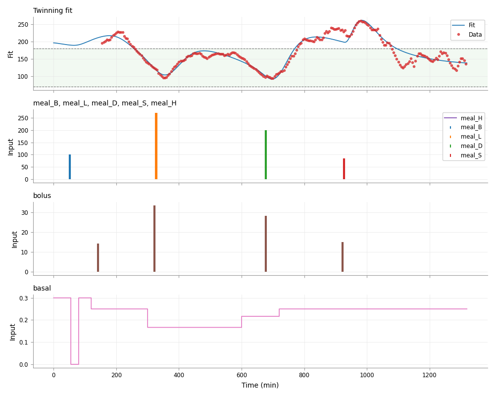
Shows how well the fitted model reproduces the observed data.
from py_replay_bg.utils.plot_twinning import plot_twinning

fig = plot_twinning(rbg_data, model, theta=result['theta'],
                    input_groups=[[0, 1, 2, 3, 4], [5], [6]],
                    thresholds=[70, 180], mask_inputs=mask_inputs)
fig.show()
- Top subplot — the simulated model
outputfor the estimatedtheta(line) vs. the observed datarbg_data.yat the non-missing indices (markers), with the threshold band. - Input subplots — the inputs that drove the fit.
plot_twinning resets and simulates the model you pass: with theta given it
resets the model with those parameters; with theta=None it uses model.theta0.
Either way the first observed glucose and the t=0 input row seed the start, as in
twinning.
Signature (abbreviated): plot_twinning(rbg_data, model, theta=None,
thresholds=None, input_groups=None, mask_inputs=None, ts_min=1.0,
output_label="Fit", observation_label="Data", figsize=None, hover=True).
For multi-day interval fits, plot_twinning_intervals(segments, ...) stitches the
per-day segments end to end into one continuous figure, with a dotted separator at
each join. segments is a chronological list of dicts, one per day, with keys
rbg_data, model and optional theta (each simulated as in plot_twinning);
the other arguments are the same as plot_twinning.
plot_replay
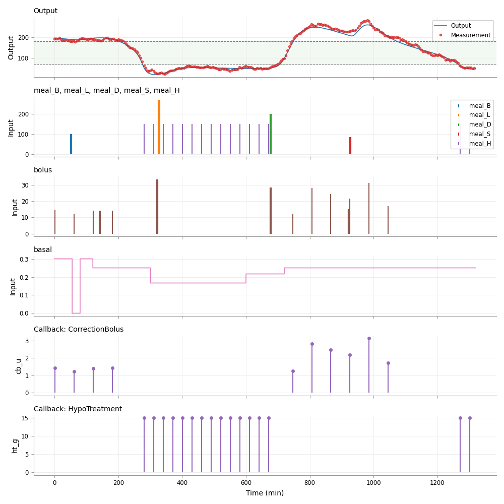
Shows the outcome of a replay.
from py_replay_bg.utils.plot_replay import plot_replay

fig = plot_replay(replay_results, thresholds=[70, 180],
                  input_groups=[[0, 1, 2, 3, 4], [5], [6]], mask_inputs=mask_inputs)
fig.show()
- Top subplot — the replayed
output(line) and, when a sensor was used, themeasurementsamples (markers), with the threshold band. - Input subplots — the applied input channels.
- Callback subplots — one per distinct callback that logged an action,
stemming the logged value
action_fieldat each action. By default (action_field=None) it is resolved per callback to the first numeric field it logged other thank/callback— e.g.cb_u(correction-bolus units) forCorrectionBolus,ht_g(rescue-carb grams) forHypoTreatment.
Signature (abbreviated): plot_replay(replay_results, thresholds=None,
input_groups=None, mask_inputs=None, action_field=None, ts_min=1.0,
output_label="Output", measurement_label="Measurement", figsize=None,
hover=True).
For multi-day interval replays, plot_replay_intervals(replay_results_list, ...)
stitches the per-day dicts returned by replay() (a chronological list) into one
figure, offsetting each segment's actions onto the glued axis. Measurement markers
are shown only when every segment carries a sensor measurement.
plot_twinning_history
When you twin with log_history=True, this shows the optimisation trajectory —
useful to sanity-check convergence.
from py_replay_bg.utils.plot_twinning_history import plot_twinning_history

if result['history'] is not None:
    plot_twinning_history(result['history'],
                          param_names=list(unknown_parameters_prior.keys()))
history is the dict recorded by the twinner, with keys theta, log_prior,
log_likelihood and log_posterior (one entry per function evaluation).
param_names labels the parameter traces (default theta_0, theta_1, ...).
- Parameter trajectory — each unknown parameter's value per function evaluation.
- Log-prior / log-likelihood / log-posterior — the three terms the twinner is optimising, one subplot each. The x-axis is the function evaluation, not time.
Interactive hover
All plotting functions attach an interactive readout by default (hover=True):
hovering any subplot drops a vertical cursor across the whole stack and reports the
values at that time/evaluation. It is ignored on non-interactive backends.