Single Meal Blueprint¶

The single-meal blueprint pairs SingleMealT1DModel with SingleMealT1DData. Use it to twin a portion of data that contains just one main meal — e.g. a breakfast, a lunch, a dinner, or a snack — spanning no more than about 8 hours.

Usage¶

from py_replay_bg.data.single_meal_t1d_data import SingleMealT1DData
from py_replay_bg.model.single_meal_t1d import SingleMealT1DModel

rbg_data = SingleMealT1DData(data=df, body_weight=100, environment=rbg.environment)
model = SingleMealT1DModel(u2ss=rbg_data.u2ss, tsteps=rbg_data.tsteps)

The data class ignores the cho_label column here (all carbs are treated as a single meal), and the model exposes a single insulin sensitivity SI. Its input channels (data_to_input) are: meal, bolus, basal, forcing_ip, forcing_ra.

Pass a 0-based index

Unlike the multi-meal data classes, SingleMealT1DData does not reset the DataFrame index and looks rows up by label. Pass a frame with a default 0-based RangeIndex (e.g. df.reset_index(drop=True) after slicing).

Structure¶

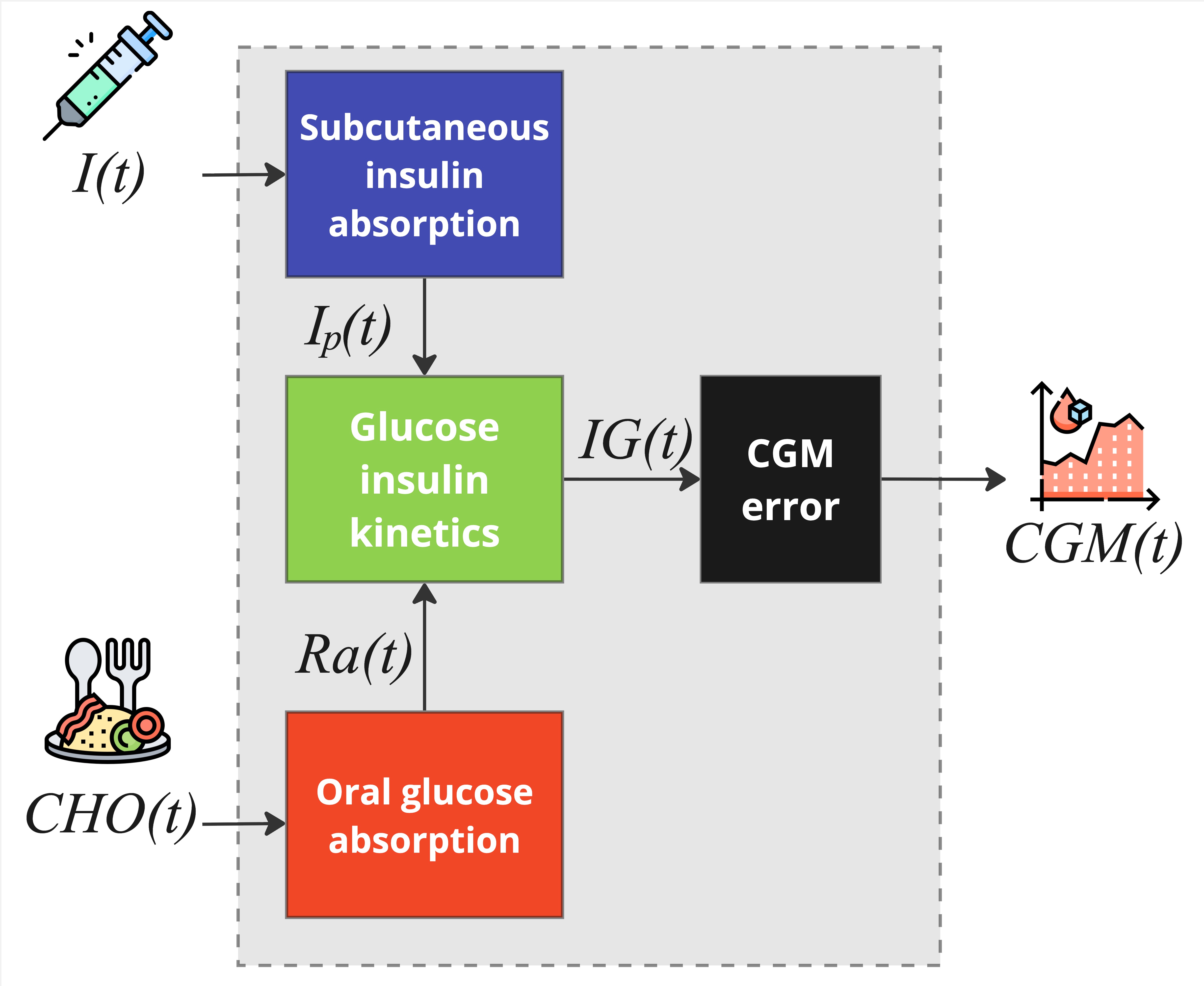
The single-meal blueprint is composed of three physiological subsystems — subcutaneous insulin absorption, oral glucose absorption, glucose–insulin kinetics — plus a CGM sensor error model applied at replay.

Single-meal blueprint

Subcutaneous insulin absorption¶

A three-compartment description of exogenous insulin infusion reaching plasma:

\[ \begin{cases} \dot{I}_{sc1}(t) = - k_d \cdot I_{sc1}(t) + I(t-\tau) \\ \dot{I}_{sc2}(t) = k_{d} \cdot I_{sc1}(t) - k_{a2} \cdot I_{sc2}(t) \\ \dot{I}_{p}(t) = k_{a2}\cdot I_{sc2}(t) - k_e \cdot I_p(t) + F_{ip}(t) \end{cases} \]

where \(I(t)\) is the bolus + basal insulin input (mU/kg/min); \(I_{sc1}\), \(I_{sc2}\) (mU/kg) are insulin in the non-monomeric and monomeric state; \(I_p\) (mU/kg) is plasma insulin; \(k_d\) is the diffusion rate; \(k_{a2}\) the absorption rate; \(k_e\) the clearance rate; \(\tau\) the insulin delay (integer minutes; for \(t < \tau\) the input is held at the basal steady state \(u_{2ss}\)); \(F_{ip}\) the forcing_ip channel (zero unless you set it).

Oral glucose absorption¶

A three-compartment gastro-intestinal tract (two stomach compartments plus the gut where CHO is absorbed):

\[ \begin{cases} \dot{Q}_{sto1}(t) = - k_{empt}\cdot Q_{sto1}(t) + CHO(t-\beta) \\ \dot{Q}_{sto2}(t) = k_{empt}\cdot Q_{sto1}(t) - k_{empt}\cdot Q_{sto2}(t)\\ \dot{Q}_{gut}(t) = k_{empt}\cdot Q_{sto2}(t) - k_{abs}\cdot Q_{gut}(t) \end{cases} \]

The rate of glucose appearance in plasma is \(Ra(t) = f\cdot k_{abs} \cdot Q_{gut}(t)\), with \(f\) the fraction of intestinal content absorbed, \(k_{empt}\) the gastric-emptying rate, \(k_{abs}\) the intestinal-absorption rate, and \(\beta\) the meal-absorption delay (integer minutes; zero input for \(t < \beta\)). \(CHO\) is the meal channel (mg/kg/min).

Glucose–insulin kinetics¶

\[ \begin{cases} \dot{G}(t) = - [SG + \rho(G) X(t)] \cdot G(t) + SG \cdot G_b + (Ra(t) + F_{ra}(t)) / V_G \\ \dot{X}(t) = - p_2 \cdot [X(t) - \frac{SI}{V_I}\cdot(I_p(t)-I_{pb})] \\ \dot{IG}(t) = - \frac{1}{\alpha}(IG(t) - G(t)) \end{cases} \]

where \(G\) (mg/dl) is plasma glucose, \(X\) the insulin action, \(IG\) the interstitial glucose (the CGM-observable signal and the model output), \(SG\) the glucose effectiveness, \(G_b\) the basal glucose, \(V_G\) the glucose distribution volume, \(p_2\) the insulin-action rate, \(SI\) the insulin sensitivity, \(V_I\) the insulin distribution volume, \(I_{pb} = u_{2ss}/k_e\) the basal plasma insulin, \(F_{ra}\) the forcing_ra channel, and \(\alpha\) the plasma-to-interstitial lag.

\(\rho(G)\) is a risk function that increases insulin action below \(G_b\):

\[ \rho(G) = \begin{cases} 1 & \text{if } G \ge G_b \\ 1 + 10\, r_1 \left[\ln(G)^{r_2} - \ln(G_b)^{r_2}\right]^2 & \text{if } 60 \le G < G_b \\ \rho(60) & \text{if } G < 60 \end{cases} \]

It is evaluated at the previous step's glucose (the model is integrated with backward Euler at a 1-minute step).

Parameter vector¶

You choose which parameters twinning estimates through unknown_parameters_prior. The example below estimates:

\[\boldsymbol{\theta}_{phy} = [k_{empt}, k_{abs}, \beta, k_{a2}, k_{d}, f, p_2, G_b, S_G, SI]^T\]

Every other parameter keeps its default, set in the model's reset (alpha, tau and beta are integer-valued):

Parameter	Default	Parameter	Default
`f`	0.9	`ka2`	0.014
`VG`	1.45	`kd`	0.026
`VI`	0.135	`ke`	0.127
`alpha`	7	`tau`	8
`SI`	10.35e-4 / `VG`	`kabs`	0.012
`SG`	2.5e-2	`kempt`	0.18
`Gb`	119.13	`beta`	0
`p2`	0.012	`r1`	1.4407
		`r2`	0.8124

What can I do with it?¶

You can create a digital twin from a portion of data that contains exactly one main meal and spans no more than ~8 hours, because the equations represent a single meal absorption (\(k_{empt}, k_{abs}, \beta\)) and a single value of insulin sensitivity.

On a cold start the insulin compartments start at the basal steady state, the gut is empty and \(X = 0\); only \(G\) and \(IG\) are seeded with the first observed CGM value. So pick a starting point sufficiently far (e.g. ~4 hours) from the last recorded insulin/meal input. See Choosing Data for Twinning.

Example¶

A complete single-meal twinning example lives in example/twin_single_meal.py:

from py_replay_bg.data.single_meal_t1d_data import SingleMealT1DData
from py_replay_bg.model.single_meal_t1d import SingleMealT1DModel
from py_replay_bg.distributions import Normal, Gamma, LogNormal, Uniform
from py_replay_bg import ReplayBG

rbg = ReplayBG()
rbg_data = SingleMealT1DData(data=df, body_weight=100, environment=rbg.environment)
model = SingleMealT1DModel(u2ss=rbg_data.u2ss, tsteps=rbg_data.tsteps)

unknown_parameters_prior = {
    'Gb':    {'prior': Normal(mu=119.13, sigma=7.11),       'min': 70, 'max': 150},
    'SG':    {'prior': LogNormal(mu=-3.8, sigma=0.5),       'min': 0,  'max': .5},
    'p2':    {'prior': Normal(mu=0.11, sigma=0.004),        'min': 0,  'max': .5},
    'f':     {'prior': Normal(mu=0.8, sigma=0.05),          'min': 0,  'max': 1},
    'ka2':   {'prior': LogNormal(mu=-4.2875, sigma=0.4274), 'min': 0,  'max': .5},
    'kd':    {'prior': LogNormal(mu=-3.5090, sigma=0.6187), 'min': 0,  'max': .5},
    'kempt': {'prior': LogNormal(mu=-1.9646, sigma=0.7069), 'min': 0,  'max': .75},
    'SI':    {'prior': Gamma(alpha=3.3, beta=1 / 5e-4),     'min': 0,  'max': .1},
    'kabs':  {'prior': LogNormal(mu=-5.4591, sigma=1.4396), 'min': 0,  'max': .5},
    'beta':  {'prior': Uniform(a=0, b=60), 'min': 0, 'max': 60, 'integer': True},
}

result = rbg.twin(rbg_data=rbg_data, model=model,
                  unknown_parameters_prior=unknown_parameters_prior,
                  parallelize=True, n_jobs=-1, n_starts=16, log_history=True)